The Signficicance of Statistical Significance

Last year, an aunt was diagnosed with extremely low bone density. She had been complaining of back pain and weakness, and a few tests later, her orthopedic confirmed that bone density was the problem. She was put on a course of medication, and then was given by shots. A year later, she got her bone density tested again, and found that there was not much improvement.

She did a few rounds of the doctors again – orthopedics, endocrinologists and the like, and the first few were puzzled that the medication and the shots had had no effect. One of the doctors, though, saw something others didn’t – “there is no marked improvement, for sure”, he remarked, “but there is definitely some improvement”.

Let us say you take ten thousand observations in “state A”, and another ten thousand in “state B”. The average of your observations in state A is 100, and the standard deviation is 10. The average of your observations in state B is 101, and the standard deviation is 10. Is there a significant difference between the observations in the two states?

Statistically speaking, there most definitely is (with 10000 samples, the “standard error” given a standard deviation of 10 is 0.1 (10 / sqrt(10000) ), and the two sets of observations are ten standard errors apart which means that the difference between them is “statistically significant” to a high degree of significance. The question, however, is if the difference is actually “significant” (in the non-statistical sense of the word).

Think about it from the context of drug testing. Let us say that we are testing a drug for increasing bone density among people with low bone density (like my aunt). Let’s say we catch 10000 mice and measure their bone densities. Let’s say the average is 100, with a standard deviation of 10.

Now, let us inject our drug (in the appropriate dosage – scaled down from man to mouse) on our mice, and after they’ve undergone the requisite treatment, measure the bone densities again. Let’s say that the average is now 101, with a standard deviation of 10. Based on this test, can we conclude that our drug is effective for improving bone density?

What cannot be denied is that one course of medication among mice produces results that are statistically significant – there is an increase in bone density among mice that cannot be explained by randomness alone. From this perspective, the drug is undoubtedly effective – that there is a positive effect from taking the drug is extremely highly likely.

However, does this mean that we use this drug for treating low bone density? Despite the statistical significance, the answer to this is not very clear. Let us for a moment assume that there are no competitors – there is no other known drug which can increase a patient’s bone density by a statistically significant amount. So the choice is this – we either not use any drug, leading to no improvement in the patient (let us assume that another experiment has shown that in the absence of drugging, there is no change in bone density) or we use this drug, which produces a small but statistically significant improvement. What do we do?

The question we need to answer here is whether the magnitude of improvement on account of taking this drug is worth the cost (monetary cost, possible side effects, etc.) of taking the drug. Do we want to put the patient through the trouble of taking the medication when we know that the difference it will make, though statistically significant, is marginal? It is a fuzzy question, and doesn’t necessarily have a clear answer.

In summary, the basic point is that a statistically significant improvement does not mean that the difference is significant in terms of magnitude. With samples large enough, even small changes can be statistically significant, and we need to be cognizant of that.

Postscript
No mice were harmed in the course of writing this blog post
The NRN premium is over

With the resignation of Infosys President BG Srinivas and the subsequent drop in the share price in the markets today, the NR Narayana Murthy premium on the Infosys stock is over. Ironically, this happens almost exactly a year since NRN made a comeback to the company in an executive capacity.

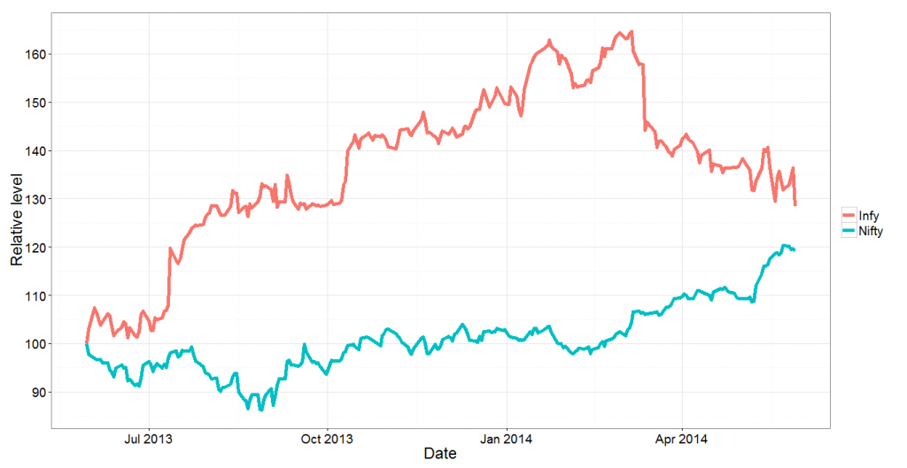
The figure below charts how the Infosys stock and the market index (Nifty ) have moved in the last one year. In order to compare the two, we have indexed their prices as of 30th May 2013, just before NRN’s return was announced (the announcement was made as of 2nd June, but the sharp spike in Infy on 31st May 2013, when the broad market fell, can be attributed to insider trading by people in the know), to 100. Notice how the Infosys stock soared in the six months after NRN’s return. In January and February, the stock traded at a 60% premium to its pre-NRN value, while the nifty was practically flat till then.

infy1

And then things started dropping. Even when the broad markets rose in March-April this year, Infosys continued to fall. The rally in early-mid May took it along, but now the stock has fallen again. This morning (latest data as of noon), the stock has fallen by about 6% thanks to Srinivas’s departure, and we can see that the gap between Infy and the market has really narrowed.

Next, we look at the ratio of the Infy price to the market index. Again we index it to 100 as of 30th May 2013. This graph shows the premium in the Infy share price over the last year. Notice that for the first time, the premium has fallen below 10% (it’s currently 7%). 

infy2


Finally, we will compare the Infy stock to the CNX IT index, which tracks the sector (that way, any sectoral premium in Infy can be extracted out). Again, we will plot the relative values of Infy to the CNX IT index, indexed to 100 as of 30th May 2013.

infy3

This graph looks like no other. What this tells us is that whatever premium Infosys enjoys over the broad market is a function of the sector, and that ever since the sharp drop in early March (on account of weak results), the NRN premium on the Infy stock relative to the sector has disappeared. As of now, compared to the sector, Infy is at an all time low.

Finally, a regression. If we regress infy stock returns against the returns in the IT index and Nifty, what we find is that Nifty returns hardly affect Infosys returns (R^2 of 7%), while the IT Index returns explain about 76% of Nifty returns. When regressed against both, Nifty returns come out as insignificant and the R^2 remains at 76%.

Putting all these statistics aside, however, the message is simple – the NRN premium on the Infy stock is over.


High Frequency Trading and Pricing Regulations

It all began with a tweet, moments ago. Degree Raju, a train travel attempter (I don’t know how often he manages to actually travel since he never seems to get tickets) tweeted this:

It is an apt analogy. The reason high frequency trading exists is that there is regulation on what the minimum bid-ask spread needs to be – it needs be at least 1 cent in the US, and at least 5 paise in India (if I’m not wrong). If the best bid (quote to purchase a stock) is at 49.95 and the best ask (quote to sell a stock) is at 50.00, there is nothing you can do to get ahead of the guy who has bid 49.95 – for regulations mean that you cannot bid 49.96!

The consequence of this is that if you want to offer the best bid, at a price close to 49.95, there is no option but for you to be the first person to have bid that amount! And so there is a race among all possible bidders, and in order to win the race you need to be fast, and so you co-locate your servers with the exchange, and so you (and your co-runners) indulge in what is called High Frequency Trading (this is a  rather simplified explanation, and it works).

Tatkal ticket booking has a similar pricing anomaly – the cancellation charges on Indian railways are fixed, and really low. Moreover, fares are static, and are not set according to demand and supply. More moreover, the Indian Railways suffers from chronic under-capacity. The result of all this together is that if you need to get a railway ticket, you should be the first person to put a bid (at a fixed price, of course) for that ticket, and so there is a race among all ticket-buyers!

In case the pricing of railway tickets was more flexible – either dynamic pricing according to demand, or higher cancellation charges (as I’ve noted here), this mad race (pun intended) to buy tatkal tickets would not be there. The way things are going I wouldn’t be surprised if agents want to get servers co-located with IRCTC servers so that they can procure tickets the fastest.

With HFT in stock prices, if only there were no limit on the minimum tick size – let’s say that a bid or an ask could just be any real number within a reasonable (say 6-digits?) precision, then in order to have the best bid, you need not be the fastest – you can compete on price!

Thus, HFT in stock markets and tatkal ticket booking are two good examples of situations where onerous regulations have led to a race to be the fastest.

And all this ties in with this old theory I have which says that the underlying reason for most financial innovation is stupid regulations. Swaps were invented because the World Bank could not borrow with floating (or was it fixed?) interest rates. CDOs became popular because AAA rated instruments required lower capital provisioning than home loans. Such examples are plentiful..

New Comment Policy

For about three or four years now the quality and quantity of comments on this blog has dropped. Earlier, there used to be some rather insightful discussions here in the comment section. Nowadays, people don’t seem to leave too many comments here. And I’m also a guilty party – for one I don’t promptly reply to comments on my blogposts, and I don’t usually leave comments on others’ blogs – preferring to add my two naya paise over twitter instead.

Also, of late I’ve been getting a lot of anonymous and sometimes abusive comments. So far I had tolerated them but henceforth will be marking all such comments as spam. Essentially I’ll be following a simple rule – if you leave a comment without leaving your name the comment will not be seen here for way too long. That will also be the case in case I feel that the comments are not adding to the discussion.

The best thing you can do while leaving a comment is to login – openid has been enabled and you can use the login of your own blog to leave the comment here. Next best thing is to leave your valid email id. If your comment follows neither of the above two conditions it will not be approved.

Thanks.

Why Keynes’s prediction has not come true

Writing in the 1930s economist John Maynard Keynes predicted at at the “time of our grandchildren” (figurative term since he himself had no kids) people would live a life of leisure and work for an average of fifteen hours a week. Yet, it’s been eighty years since and we still slog away, putting in anywhere between forty and sixty hours a week as we earn our living. And it doesn’t look like things are going to change soon

So why did this happen? I propose two reasons. When I quit my first job almost eight years ago within three months of joining I complained that the workload was way too high. I added that I didn’t need all the money that job paid me and wouldn’t mind taking up something that paid half the money and where I had to work only half the time. No such thing materialized and I slogged away, before going freelance two years back.

Now why does this little anecdote matter? I’m using this to show that the returns to work are not linear. If you were to plot the number of hours worked per week on the x axis and the total value added on the y axis you are likely to get a convex function. In other words the marginal benefit out of every additional hour you work per week is an increasing function of how much you’ve already worked.

The question is why this is so. One simple answer is that in jobs with a high degree of learning by working longer you end up learning faster. Then within the job you can have network effects where the work you do in one part of the job can help you do another part better (I constantly see this in my freelancing where I work on several projects at a time). If there is a steep learning curve it is easier for the firm to appoint one worker to work sixty hours a week than two to work thirty each – since the starting costs get saved. And so forth.

So this increasing returns to effort (in terms of the hours worked) is that the trade off between work and leisure gets resolved in favour of leisure only at a very high level of work – where you are working close to capacity and don’t want to risk burnout and want to maintain your sanity. Before that the increasing returns to effort means that you are likely to put off leisure in favour of “just a little more work”.

The question is if all jobs work this way, and why an economist as brilliant as Keynes didn’t see this concept of increasing returns to work. The answer is that increasing returns to work applies only to a certain kind of jobs – jobs that require a high level of skill and learning and which can be broadly classified as “knowledge jobs”.

Back in Keynes’s time such knowledge jobs were few – far fewer than they are today. Most workers were in jobs that didn’t require a high degree of skill or learning. In unskilled jobs or jobs that are physically demanding the expanding returns to effort part of the curve is extremely short. Once you have figured out the best way to bolt together two metal pieces doing more of this job is not going to make you much faster in bolting together two metal pieces.

Instead since it is physical after you’ve put in a certain number of hours in a day you begun to tire and become less efficient (notice this point occurs at a later stage for knowledge jobs). And the returns to hours curve starts flattening out much sooner. If you were to do the trade off with leisure using such a curve the equilibrium might occur much earlier than for knowledge work – perhaps at Keynes’s predicted value of fifteen hours per week.

Now even today while the proportion of non knowledge jobs is smaller than eighty years back the number of people doing such jobs is not small. So if the work-leisure equilibrium happens at fifteen hours a week why do people work longer?

The answer is that work-leisure is not the only equilibrium one is solving for. You also need to work enough to be able it fund your living. And it has happened that fifteen hours of non knowledge work pays nowhere close tO what is required to fund a reasonable living. For this reason non knowledge workers are forced to work much longer than their work-leisure equilibrium rule permits!

So why didn’t Keynes see this? I think what he missed was the boom in the knowledge economy in the postwar period. With the rise in the knowledge economy what you had was a set if jobs that had increasing returns to effort. Moreover these returns, on an hourly basis, were far larger than the returns on a non knowledge job. The boom in the knowledge economy meant that people working in such jobs impacted general prices and this forced the non knowledge workers to work longer!

So we have the unique situation now that those people who can afford to work for only fifteen hours a week have no incentive to do so. On the other hand people who have an incentive to work no more than fifteen hours a week are forced to work longer because otherwise they cannot find their lives!!

Money can buy me Premier League performance

The following graph plots the premier league performance (in terms of points) for the 2012-13 season as a function of the team’s wage bill. Apart from a few outliers here and there the correlation is astounding:

wageperformance


The red line is the line of best fit (according to a linear regression) and comparing team standings with respect to the line shows how well teams performed relative to what their wages would predict.

It is interesting to see that Manchester City almost fall off the charts in terms of wages, yet they could not translate this to on-pitch performance. It can also be seen that Manchester United, Spurs and Everton significantly over-performed given their wage bills.

Based on the wage bill, it would have also been reasonably easy to predict that Wigan Athletic and Reading would get relegated at the end of the season – though it must be mentioned they underperformed their wage bills, but QPR should have done a lot better given the size of their pay packet.

A simple linear regression of points against wage bill shows that every GBP 4 million increase in the wage bill leads to one additional point in the premier league! And the regression has an R-square of 69% – which means that the team’s wage bill can predict 69% of the variation in the team’s performance! Which is extremely significant.

The screenshot of the regression is given below: wagerank


Note that in this post we only use the wage bill and not any transfer fees paid. However, the assumption is that the two are reasonably correlated and we are not losing out on any information by using only the wage bill.


Classifying cricket grounds

For some work I’m trying to classify cricket grounds. The question is if we can classify cricket grounds based on what kind of cricket they support. Some pitches are slow and low – it is hard to score runs, but also hard to get the batsman out. Some others are fast and bouncy – easy to score and easy to get out. Then you have the “batting pitches” – easy to score and hard to get out and “bowling pitches” – hard to score but easy to take wickets.

Essentially I’m trying to see if I can classify a ground into one of the above four regimes (or a superposition of them) at different stages in a game – this will help estimate how the rest of the game is going to play out.

For this, I was looking at the runs per ball and balls per wicket statistic for a number of grounds based on T20 matches. All grounds which hosted over 10 T20 matches (international or IPL) before the 10th of April have been considered for this analysis. It is interesting, to say the least.

Here is the scatter plot – bottom right (only the Oval) is easy to score, easy to get out. Top right are the batting pitches, bottom left the bowling pitches and top left the slow-and-low! It is interesting that the “most bowling pitch” of the lot is Chittagong! The only Indian ground that can be classified thus is DY Patil Sports Academy in Navi Mumbai!

t20grounds

The long-term effects of government failure

In a good blog post on FirstPost, R Vaidyanathan writes that one of the possible reforms for the new government to take up would be to invest massively in electricity and water supply infrastructure and ensure 24 x 7 supply of these two commodities throughout the county. In his post, he explains that a move such as this will help Indian households (especially “middle class” households) and industry save a sum total of Rs. 1 lakh crore per year. While his numbers are not particularly convincing, his point is well taken – that irregular supply of basic infrastructure leads to additional private investment in such infrastructure which is an unnecessary cost. Electricity and water supply have “natural monopolies” and it helps to have a single supplier (in a local area at least) supply these goods rather than people making their own private supply arrangements.

Setting aside the problem of creating capacity for 24 x 7 universal power and water supply (priced at marginal cost, I assume), the problem reform such as this is likely to face is that there will be entrenched players who have a vested interest in such reform not taking place. And the  reason such vested interests exist is because of past government failure.

In the absence of reliable public supply of infrastructure, private companies have come up to fill in the gaps. You have, for example, companies that manufacture invertors (to store and supply electricity in times of power failure), those that manufacture diesel generators, companies that supply water in tankers when there is none in the pipes (or worse, pipes don’t exist) and so  forth. None of these companies will like the reform that Vaidya has proposed – for reliable supply of water/power will put them out of business! Hence they can be expected to lobby against such reform! Notice that the primary reason such companies exist is because of past government failures. Had past governments intervened and invested at the right time to provide reliable power and water supply, there would have been no gap in the market for such companies to fill.

Power and water supply are only two of several examples. Take for example the basic public good of law and order (strictly speaking power and water supply are not public goods). The lack of effective law and order enforcement by the state governments has led to a mushrooming of private security agencies. Every apartment building, every office building, malls and hotels are all now patrolled by a heavy posse of private security guards. In the presence of effective policing, these agencies have no business being in business (except perhaps in very limited cases)!

The point I’m getting at is that government failure at a particular point in time can lead to continued government failure. When we encounter policy paralysis, it is not just a temporary slowdown in decision-making and policy-making we face – it can lead to significant long-term consequences.

Here is an old related blog-post on my personal blog on private supply of what should be provisioned by the government.


Exponential need not mean explosive

Earlier on this blog I’ve written about the misuse of the term “exponential” when it is used to describe explosive increase in a particular number. My suspicion is that this misuse of the word “exponential” comes from Computer Science and complexity theory – where the hardest problems to crack are those which require time/space that is exponential in the size of the data. In fact, the entire definition of P, NP and NP-completeness have to do with the distinction between problems that take exponential resources versus those that take resources that are a polynomial function of the size of data.

Earlier today, I shared this blog post by Bryan Caplan on Puerto Rican immigration into the United States with a comment “exponential immigration”. I won’t rule out drawing some flak for this particular description, for Caplan’s thesis is that Puerto Rican immigration took a long time indeed to “explode”. However, I would expect that the flak I get for describing this variable as “exponential” would come from people who mistake “exponential” for “explosive”.

Caplan’s theory in the above linked blog post is that immigration from Puerto Rico to the United states was extremely slow for a very long time. It was in the late 1890s that a US Supreme Court ruling allowed free access to Puerto Ricans to the United States. However, it took close to a hundred years for this immigration to “explode”. Caplan’s theory is that the number of people moving to the US per year is a function of the number of Puerto Ricans who are already there!

In other words, the immigration process can be described by our favourite equation: dX/dt = kX, solving which we will get an equation of the form X = a exp(kt), which means that the growth is indeed exponential in time! Yet, given a rather small value of X_0 (the number of Puerto Ricans in the United States at the time the law was passed), and given a small value of k, the increase has been anything but explosive, despite it being exponential!

The point of this post is worth reiterating: the word “exponential”, in its common use, has been taken to be synonymous with “explosive”, and this is wrong. Exponential growth need not be explosive, and explosive growth need not be exponential! The two concepts are unrelated and people would do well to not confuse one with the other.


Analyzing IIMA Admissions

In response to an RTI query, IIM Ahmedabad has disclosed the cutoff percentiles across various categories for getting a seat in IIMA. Before we analyze further, there are two points to be noted. Firstly, what has been disclosed is the “minimum cutoff percentile”, which means that at least one student with that percentile score was admitted to IIMA in that year. It gives us no information on the “average percentile score” for admitted students belonging to that particular category. Secondly, CAT percentile is only one of the criteria used for admission into IIMs. A response by IIM Bangalore a few years back to an RTI query showed that the CAT percentile has only a 15% weight in the entire admission process (the rest going to 10th and 12th standard board exam scores, college CGPA, performance in interviews and the like). Given these two conditions, we should look at the following analysis with a bit of salt.

First up, here is a graph showing the minimum percentile among admitted students of various categories over the years:

Rplot


There are a few things that stand out from this graph:

1. The cutoff percentage for general category students has been consistently high. Despite a comprehensive set of factors being used for admissions, if you belong to the general category, a high CAT percentile is a necessary condition to join IIMA

2. Reservations for Other Backward Classes (OBCs) happened in a phased manner. In the first year (2008) only about 5% of the seats were reserved for students from these classes. This has been gradually ramped up to the statutory 27.5%. In the initial years, after reservation for OBCs was imposed, commentators mentioned that their cutoff was not much lower than that for general category students and so there would be no dilution in quality. However, the data above shows that it was a function of the extent of reservation that the cutoffs were similar. If CAT percentile is to be taken as a general statement of an MBA student’s quality, reservation for OBCs has definitely led to dilution.

3. There is massive volatility in cutoffs for SC/STs. It must be noted here that the percentile scores are national – percentiles for students from different categories are not disclosed separately. It seems like the quality of applicants belonging to SC/ST categories has been varying significantly over the years. One year (2008/09) SC/ST students need to be in top 10% of all applicants to gain admission into IIMA. In another (2013) students belonging to ST category need to beat only 40% of all applicants to get in! This is bizarre, and it brings us to..

4. Students from ST category getting admission with 40 percentile in CAT in 2013 is plain absurd. What makes it more absurd is that more than half the students who attempted CAT in 2013 got ZERO or less (remember that CAT has negative marking). Maybe there was a real dearth of applicants from the ST category last year but what this tells us is that someone who got an overall negative score in CAT got admission into IIMA last year. Actually this is beyond bizarre.

5. Time for a personal anecdote. Close to 20 out of the 180 odd people who started at IIM Bangalore with me (2004-06) did not make it to the second year, based on their performance in the first year. About half of those were put on a “slow track programme” and finished their MBA in three years. The other ten did so badly they were asked to repeat the first year in full, without concessions. From what I remember all of them eventually dropped out. A large proportion of these twenty who did not make it past the first year belonged to SC/ST categories. I must also mention here that there was a significant number of students from these categories that did rather well and finished close to the top of the batch.

While it might be seen as an act of nobility to give admission in a premier college to someone with a low score but from a historically underprivileged background, the impact on their careers must also be taken into account. All said and done, the flagship course in IIMs is a rather tough course, and it is not difficult to fall behind. What is the use of giving someone admission only for him to fail and eventually drop out? Would he not have been better off continuing in his pre-MBA job rather than having his career disrupted by admission to a premier institute and subsequent failure?

All this said, it would make sense for someone in an IIM (a professor involved in admissions, perhaps) to do an analysis of correlation of CAT scores with performance at IIMs (I understand that one of the reasons the weight of CAT score was  reduced was that one such study revealed CAT score was less of a predictor of IIM performance than high school and undergraduate scores). An analysis such as that might reveal that there is an absolute lower cutoff in terms of performance in CAT such that students scoring lower are extremely unlikely to do well. It might give a case for reassessment of the affirmative action policies.